Date:2026-02-10
Ordered Dithering (Bayer) in Processing : From Basics to Levels
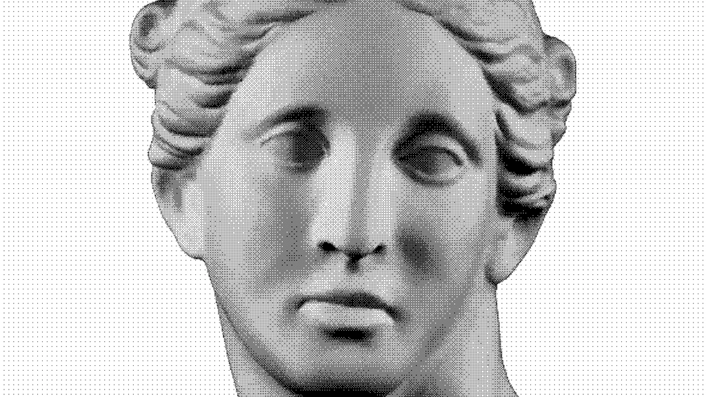
Dithering is a classic technique that smooths images when colors are limited. While it may seem like simple black-and-white conversion, it drastically improves the appearance of gradients and textures.

This article focuses on one of the most fundamental dithering methods: Ordered Dithering. It provides working Processing code, explains the meaning of the Bayer matrix (the “order of becoming white”), and organizes how to handle the characteristic “pattern look” that ordered dithering produces.
The complete sample code for this article is available for download on Patreon.
☕ Support my Work:) / Coffee Supplier on Patreon
1. What is Dithering?
Dithering is a technique that uses human visual perception to represent intermediate tones even when the output device can display only a limited number of colors (or tonal levels).
For example, in a situation where only two values (black and white) are possible, if the image is converted with a simple threshold like “brightness > 128 → white,” smooth gradients become broken into step-like segments and lose their softness. This is called posterization or banding, and it becomes especially visible in areas such as skies or shadows where brightness changes slowly.
In contrast, if black and white pixels are intentionally distributed, they may appear as “grain” or “patterns” up close, but from a slightly farther distance they visually average out and are perceived as intermediate brightness. In other words, even though no true mid-tone exists on the screen, the visual system completes the missing tone by spatial averaging. Dithering is the technique of designing this perceptual “illusion.”
This idea is closely related to halftoning used in newspapers and magazines. In print, continuous ink density is difficult to control, so tonal values are represented by dot density and dot arrangement. Dithering can be seen as transferring this halftone concept into digital images and implementing it as a pixel-level algorithm.
It is also important that dithering is not merely an “old low-resolution effect.” Even today, dithering is used for purposes such as:
- Low bit-depth displays (e-ink, embedded displays, LEDs, etc.)
- Compression or simplification (artistic black-and-white / limited-color looks)
- Avoiding banding (converting smooth gradients into controlled grain)
- Texture design in generative expression (patterns, noise, retro aesthetics)
In other words, dithering is not only a way to overcome technical constraints, but also a method for designing the appearance of images themselves.
This article starts with one of the most basic and easy-to-implement forms: Ordered Dithering, and explains it through working Processing code.
2. What is Ordered Dithering?
There are several families of dithering, but Ordered Dithering has the following characteristics:
- Quantizes pixels into black/white (or a small number of tones)
- Uses thresholds that vary by pixel position instead of being constant
- Produces tonal representation through a regular pattern
In normal binary thresholding, the same threshold is applied everywhere (for example, “brightness > 128 → white”). In ordered dithering, the threshold changes depending on pixel position.
In other words, the idea is:
“Decide in advance how easily each position becomes white.”
As a result, when image brightness increases slightly, white pixels do not increase as a solid block. Instead, they increase while being spatially scattered. This is why ordered dithering can visually produce gradients even in black and white.
Ordered dithering is computationally light and simple to implement, which makes it suitable for real-time use. Compared to error diffusion methods (such as Floyd–Steinberg), it tends to produce more stable grain, making it easier to use for animation and video.
3. What is a Bayer Matrix? (4×4 Example)
A well-known representative of ordered dithering is Bayer dithering. Bayer dithering uses a repeating threshold matrix (threshold map) tiled across the image:
int[][] bayer4 = {
  { 0, 8, 2, 10},
  {12, 4, 14, 6},
  { 3, 11, 1, 9},
  {15, 7, 13, 5}
};
The important point is that these numbers are not random. They represent the order in which pixels turn white. As the brightness of the image increases from 0 to 255, inside each 4×4 tile, the positions with smaller numbers turn white earlier.
By distributing this “turning white order” spatially, the algorithm prevents white pixels from clustering locally, making tones appear smoother. Because the pattern is regular, the perceived brightness tends to remain stable as an area.
4. Implementation in Processing (Bayer 4×4)
In Processing, implementing Bayer dithering generally follows these steps:
- Get brightness from the source image
- Retrieve the Bayer matrix value for that pixel position
- Use it as a threshold and convert to black/white
Below is the minimal working example:
void applyBayerDithering4(PGraphics source) {
  loadPixels();
  source.loadPixels();

  int[][] bayer4 = {
    { 0, 8, 2, 10},
    {12, 4, 14, 6},
    { 3, 11, 1, 9},
    {15, 7, 13, 5}
  };

  for (int y = 0; y < height; y++) {
    for (int x = 0; x < width; x++) {
      int loc = x + y * width;

      float b = brightness(source.pixels[loc]); // 0..255

      float t = bayer4[x % 4][y % 4];           // 0..15
      float threshold = (t / 15.0) * 255.0;

      pixels[loc] = (b > threshold) ? color(255) : color(0);
    }
  }

  updatePixels();
}
In Processing, pixels[] is a 1D array, so the 2D coordinates (x, y) must be converted into an index:
int loc = x + y * width;This loc represents “which element in pixels[] corresponds to this pixel.”
The following line tiles the Bayer matrix across the whole image:
float t = bayer4[x % 4][y % 4];x % 4 and y % 4 fold the coordinates into the range 0..3. As a result, the 4×4 Bayer matrix repeats in a tiled pattern across the screen, assigning a different threshold to each position.
The next line matches the scale:
float threshold = (t / 15.0) * 255.0;- Bayer values
tare 0..15 - brightness() values
bare 0..255
Without scaling, the comparison would not work properly. So:
- t / 15.0 normalizes 0..15 into 0..1
- multiplying by 255.0 converts it back to 0..255
Now threshold and b can be compared consistently, producing the ordered dithering effect:
- threshold varies by position
- white pixels increase in a regular scattered pattern
5-1. Extending to 8×8 / 16×16
Bayer dithering can be extended beyond 4×4 to 8×8 and 16×16. As the matrix size increases, the black/white distribution becomes finer even in areas of constant brightness, and gradients appear smoother.

- 4×4: the pattern is obvious (strong retro look)
- 8×8: the pattern becomes finer and tonal steps increase
- 16×16: even smoother, but may look blurry depending on the image
A Bayer 8×8 matrix (0..63) looks like this:
int[][] bayer8 = {
  { 0, 48, 12, 60,  3, 51, 15, 63},
  {32, 16, 44, 28, 35, 19, 47, 31},
  { 8, 56,  4, 52, 11, 59,  7, 55},
  {40, 24, 36, 20, 43, 27, 39, 23},
  { 2, 50, 14, 62,  1, 49, 13, 61},
  {34, 18, 46, 30, 33, 17, 45, 29},
  {10, 58,  6, 54,  9, 57,  5, 53},
  {42, 26, 38, 22, 41, 25, 37, 21}
};
To handle such sizes, it is often more convenient in Processing to generate Bayer matrices automatically and switch sizes as needed.
Below is an implementation example that handles 4/8/16 uniformly:
void applyBayerDithering(PGraphics source, int matrixSize) {
  if (!isPowerOfTwo(matrixSize) || matrixSize < 2) return;

  int[][] bayer = makeBayerMatrix(matrixSize);
  float maxV = matrixSize * matrixSize - 1;

  loadPixels();
  source.loadPixels();

  for (int y = 0; y < height; y++) {
    for (int x = 0; x < width; x++) {
      int loc = x + y * width;

      float b = brightness(source.pixels[loc]);
      float t = bayer[x % matrixSize][y % matrixSize];
      float threshold = (t / maxV) * 255.0;

      pixels[loc] = (b > threshold) ? color(255) : color(0);
    }
  }
  updatePixels();
}

int[][] makeBayerMatrix(int n) {
  if (n == 2) {
    return new int[][] {
      {0, 2},
      {3, 1}
    };
  }

  int half = n / 2;
  int[][] prev = makeBayerMatrix(half);
  int[][] m = new int[n][n];

  for (int y = 0; y < half; y++) {
    for (int x = 0; x < half; x++) {
      int v = prev[x][y];

      m[x][y]               = 4 * v + 0;
      m[x + half][y]        = 4 * v + 2;
      m[x][y + half]        = 4 * v + 3;
      m[x + half][y + half] = 4 * v + 1;
    }
  }
  return m;
}

boolean isPowerOfTwo(int n) {
  return (n & (n - 1)) == 0;
}
5-2. Extending to levels (Number of Tones)
So far, the output has been fixed to binary black or white.
However, dithering can also be used not only for 2 values, but also for a small number of tones (4 tones, 8 tones, 16 tones, etc.).

Here, levels means the number of quantization steps (the number of output brightness values).
- levels = 2 → binary (0 / 255)
- levels = 4 → 4 tones (0 / 85 / 170 / 255)
- levels = 8 → 8 tones
- levels = 16 → 16 tones
The role of dithering is not “increasing the number of tones.”
It is distributing banding artifacts (step-like edges) into spatial grain when reducing tones.

The essence of ordered dithering is “shifting the quantization boundaries by position.”
In the binary case, the algorithm changes the threshold that decides “white or black.”
When increasing levels, it changes the boundaries that decide “which quantization step to round to.”
This can be generalized as:
- input brightness is continuous: 0..255
- output is discrete: levels steps
- the Bayer matrix contains the “priority order” of becoming brighter
- use that order to slightly shift the quantization boundaries
Implementation in Processing (levels-enabled)
Below is an implementation that allows both Bayer matrix size (4/8/16…) and the number of tonal levels levels.
void applyBayerDitheringLevels(PGraphics source, int matrixSize, int levels) {
  if (!isPowerOfTwo(matrixSize) || matrixSize < 2) return;
  if (levels < 2) return;

  int[][] bayer = makeBayerMatrix(matrixSize);

  // Bayer values are 0..(N^2-1), but for normalization we use N^2
  float maxV = matrixSize * matrixSize;

  loadPixels();
  source.loadPixels();

  for (int y = 0; y < height; y++) {
    for (int x = 0; x < width; x++) {
      int loc = x + y * width;

      float b = brightness(source.pixels[loc]); // 0..255

      // Normalize Bayer value to 0..1
      float t = bayer[x % matrixSize][y % matrixSize];
      float d = (t + 0.5) / maxV;  // 0..1 (centered)

      // Normalize brightness to 0..1
      float bn = b / 255.0;

      // Quantize to levels (shift boundary by d)
      float q = floor(bn * (levels - 1) + d);
      q = constrain(q, 0, levels - 1);

      // Convert quantized value back to 0..255
      float out = (q / (levels - 1)) * 255.0;

      pixels[loc] = color(out);
    }
  }

  updatePixels();
}
This process can be broken into three steps:
1) Normalize Bayer values to 0..1
A Bayer matrix contains integers in the range 0..(N^2-1).
We normalize them into 0..1 and use them as a small positional offset.
float d = (t + 0.5) / maxV;The +0.5 shifts each cell value toward the center of its interval.
This reduces bias and often makes the dithering pattern more uniform.
2) Quantize brightness to levels, but shift boundaries
Normal quantization would be:
q = floor(bn * (levels - 1));But this uses fixed boundaries and tends to produce banding.
Ordered dithering shifts the boundary by the Bayer offset d:
q = floor(bn * (levels - 1) + d);This creates the effect that:
- some positions become brighter slightly earlier
- other positions become brighter slightly later
As a result, the boundary is spatially scattered and the banding becomes grain.
3) Convert quantized values back to 0..255
The quantized index q is in 0..(levels-1), so it must be mapped back:
float out = (q / (levels - 1)) * 255.0;Usage examples
You can independently control matrix size and tonal levels:
applyBayerDitheringLevels(pg, 4, 2);   // 4x4 + binary
applyBayerDitheringLevels(pg, 4, 4);   // 4x4 + 4 levels
applyBayerDitheringLevels(pg, 8, 8);   // 8x8 + 8 levels
applyBayerDitheringLevels(pg, 16, 16); // 16x16 + 16 levels
Difference between matrixSize and levels
A common confusion is that matrixSize and levels control different things.
- matrixSize: controls the fineness of the pattern
→ larger makes the pattern finer - levels: controls the number of output tones
→ larger makes the tones smoother
So if the goal is to increase smoothness of tone, increasing levels is usually more noticeable than increasing matrixSize.
6. Meaning of the Bayer Matrix: “The Order of Becoming White”
A Bayer matrix is often explained as a “threshold map,” but it is easier to understand as a priority map.
- smaller values turn white earlier
- larger values remain black until later
This causes white pixels to increase while being spatially distributed as brightness increases. As a result, even in binary black and white, intermediate tones appear to exist.
7. How to Handle the “Pattern Look” of Ordered Dithering
The biggest characteristic of ordered dithering is that it always produces a regular pattern in exchange for tonal representation. Depending on the situation, this pattern can be either a weakness or a strength.
7-1. Weakness: when the pattern becomes distracting
Regular patterns are more visible in areas such as:
- large flat regions
- slow gradients
- around thin lines and text
In these cases the image may look “processed” rather than natural.
7-2. Strength: stable in motion
Error diffusion dithering (such as Floyd–Steinberg) can cause grain to shift from frame to frame in animation, often producing a crawling effect moving toward the lower-right direction.
Ordered dithering, on the other hand, has a fixed pattern, so it tends to be visually stable for video and animation.
7-3. Using it as an aesthetic element
Instead of hiding the pattern, ordered dithering can be used intentionally as a design element:
- retro texture
- halftone-like print feel
- generative patterns
Especially in Processing, dithering often behaves less like “image processing” and more like “texture generation.”
8. Ordered dithering (Bayer)
This article covered the basics of Ordered dithering (Bayer) and implemented it in Processing.
- dithering is a technique to create the illusion of intermediate tones using limited tones
- ordered dithering changes the threshold depending on pixel position
- the Bayer matrix is a priority map that defines the order of becoming white
- 4×4, 8×8, 16×16 change both pattern and tonal characteristics
- the pattern of ordered dithering can be a drawback or an aesthetic strength
In the next article, the other major family—Error diffusion—will be covered by implementing Floyd–Steinberg dithering in Processing and comparing it with ordered dithering.
References
- Ordered dithering — Wikipedia
https://en.wikipedia.org/wiki/Ordered_dithering
9. Work Example | Sound visualization
Recommended Book / Generative art for beginner
Generative Art: A Practical Guide Using Processing – Matt Pearson
Generative Art presents both the techniques and the beauty of algorithmic art. In it, you’ll find dozens of high-quality examples of generative art, along with the specific steps the author followed to create each unique piece using the Processing programming language. The book includes concise tutorials for each of the technical components required to create the book’s images, and it offers countless suggestions for how you can combine and reuse the various techniques to create your own works.
Purchase of the print book comes with an offer of a free PDF, ePub, and Kindle eBook from Manning. Also available is all code from the book.
—–
► Generative Art: A Practical Guide Using Processing – Matt Pearson
Publication date: 2011. July
Support my Website
By using our affiliate links, you’re helping my content and allows me to keep creating valuable articles. I appreciate it so much:)
BGD_SOUNDS (barbe_generative_diary SOUNDS)
barbe_generative_diary SOUNDS will start sharing and selling a variety of field recordings collected for use in my artwork “Sound Visualization” experiments. All sounds are royalty-free.
