When handling a large number of objects, computational costs can become high, leading to decreased processing speed. This is especially true when performing collision detection or searching for nearby objects, where checking all combinations is inefficient.

In this article, we explore methods to significantly reduce computational load by utilizing spatial partitioning algorithms. Among various methods, we focus on the grid-based partitioning approach, which is relatively simple to implement.

The full sample code for this article is available for download on Patreon after following.
(It uses Processing for the implementation.)
☕ Support my Work:) / Coffee Supplier on Patreon

What is Spatial Partitioning?

Spatial partitioning is a technique that classifies objects into specific regions to reduce computational costs. Representative algorithms include:

• Grid-based Partitioning: Divides space into a grid and assigns objects to each cell.
• Quadtree: A data structure that recursively subdivides 2D space into four parts.
• Octree: A data structure that recursively subdivides 3D space into eight parts.

What is Grid-based Partitioning?

In grid-based partitioning, the simulation area is divided into cells of a specified size. Particles within each cell are managed in a list, and when calculating interactions between particles, only those in the target cell and its neighboring cells are considered. This approach reduces the number of calculations by focusing only on nearby particles, rather than all particles.

1. Determining Cell Size

Deciding the cell size (cellSize) is one of the most crucial factors in spatial partitioning. If the cell size is too large, the calculation range becomes too broad, reducing efficiency. Conversely, if it’s too small, the number of cells increases, leading to higher management overhead.

The cell size is determined based on MAX_DISTANCE (the maximum distance between particles). A suitable cellSize can be estimated using the following formula:

int range = ceil(float(MAX_DISTANCE) / cellSize);

MAX_DISTANCE	cellSize	MAX_DISTANCE / cellSize	range の理想値
100	50	2.0	ceil(2.0) = 2
100	100	1.0	ceil(1.0) = 1
100	200	0.5	ceil(0.5) = 1
150	50	3.0	ceil(3.0) = 3

2. Grid Structure

The grid is typically implemented as a two-dimensional array. The size of the array is determined by dividing the width and height of the simulation space by cellSize. Each cell contains a list of particles present in the corresponding area.

// Creating the grid
cols = width / cellSize;
rows = height / cellSize;
grid = new ArrayList[rows][cols];

// Adding particles to cells
for (int i = 0; i < MAX_PARTICLES; i++) {
   Particle p = new Particle();
   grid[int(p.pos.y / cellSize)][int(p.pos.x / cellSize)].add(p);
}

3. Neighbor Search

The advantage of spatial partitioning becomes evident when calculating interactions between particles. Each particle searches only its own cell and the surrounding cells. The search range is determined based on the previously set range. If range is 1, the particle examines its own cell and the surrounding eight cells.

In the above code, by using range, the particle searches its own cell and neighboring cells, interacting only with nearby particles.

4. Advantages and Disadvantages

Advantages

• Reduction in Computation: By focusing only on particles in nearby cells instead of comparing all particles, computational load is significantly reduced.
• Scalability: Even as the number of particles increases, the computational load does not increase drastically.
• Efficient Memory Management: Managing particles by cell improves memory utilization efficiency.

Disadvantages

• Overhead in Cell Management: There is a certain overhead in managing cells, especially when the cell size is small or the simulation space is large.
• Balance in Spatial Partitioning: If the cell size is not set appropriately, the method may not function efficiently.

5. Optimization Points

• Optimizing Cell Size: By appropriately setting cellSize based on MAX_DISTANCE, computational load can be minimized.
• Adjusting Search Range: By adjusting the value of range, the number of cells to be calculated can be controlled, further reducing computational load.
• Considering Parallelization: Since the calculation of interactions between particles is independent, utilizing parallel processing (e.g., leveraging the GPU) can achieve further speed improvements.

Comparison

Below is a comparison between cases without and with spatial partitioning, showing the frame rate when running with 10,000 particles.

Without Spatial Partitioning

With Spatial Partitioning

Recommended Book

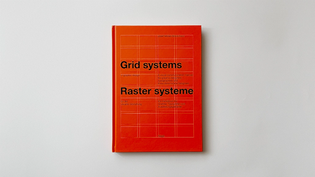
"Grid Systems in Graphic Design" by Josef Müller-Brockmann

This book discusses grid systems, a layout method that enhances design coherence and readability by arranging text and images based on continuous rows and columns. Originally conceived for print layouts, grid systems are now utilized in all design fields, including web design. Even when creating 2D graphics with tools like Processing or P5.js, there is much to learn from this system. First published in 1981.

🌐 Support my Website
By using our affiliate links, you’re helping my content and allows me to keep creating valuable articles. I appreciate it so much:)

BGD_SOUNDS (barbe_generative_diary SOUNDS)

At BGD_SOUNDS, we have started sharing and selling a collection of field recordings stocked for use in sound visualization experiments. Nearly all recordings are captured in 192kHz-32bit float quality and are royalty-free, allowing for unrestricted use. New releases are added regularly, so if you’re looking for sound sources, consider following us to stay updated.